

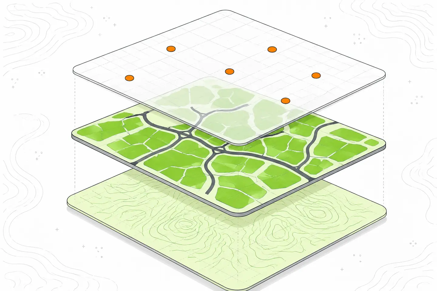
A useful first geographic information system project starts with one question, a few layers and an output you can check. This tutorial follows a simple task: mapping public facilities alongside a town boundary and roads. The same sequence applies to survey points, land cover or buildings: organise the files, inspect the data, check coordinates, style the map and verify any analysis before exporting.
Define the question and gather the data
Write down what you need to discover. “Where are the facilities?” requires a location map. “Which facilities are near a road?” requires a distance rule and a spatial operation. Decide the study area, the period represented by the data and whether the result should be a map, a table or a new dataset.
For the example, gather a point layer of facilities, a polygon layer for the town boundary and a line layer of roads. Read the accompanying metadata before using them together. Check coverage, collection dates, coordinate reference systems and any restrictions on reuse. A detailed road layer does not make an older facility inventory complete or accurate.
Organise the project files
Create separate folders for original data, working results and exports. Keep the originals unchanged. Give derived files descriptive names and record their inputs in a short notes file. Retain any accompanying files supplied with a dataset; some formats depend on several files remaining together.
Save the project early, then save after substantial changes. A project records layer references, styling and map settings; it should not be assumed to contain the underlying datasets. When sharing or moving it, include the required data and check that the saved paths still resolve.
Project-file documentation explains how map settings and data references fit together. A basic-map training module provides a useful sequence for adding vector data and reordering layers. Apply that sequence to your own small dataset before attempting a larger analysis.
Load layers and inspect their records
Use your application's data-loading controls to add one layer at a time. Zoom to each layer's extent and confirm that it covers the expected area. Arrange broad polygons below lines and points so opaque fills do not hide smaller features. Put background imagery beneath the other layers.
Open each attribute table. Geometry describes location and shape; attributes describe the feature. Identify the fields containing names, categories, dates and unique identifiers. Look for missing values, duplicate records and inconsistent category spelling. Numbers stored as text may sort or calculate differently from numeric values.
The QGIS attribute-table documentation covers viewing, selecting and filtering records. Select a facility category and check its corresponding points on the map. Distinguish a selection from a filter: highlighting records does not necessarily exclude the others from a later operation.
Check whether apparently repeated facilities are genuine duplicates or separate records at the same location. Do not delete them based on appearance alone. Compare identifiers and descriptive fields, then record any cleaning decision in the working copy.
Check coordinate reference systems
A coordinate reference system, or CRS, describes how coordinate values relate to locations on Earth. Check the CRS recorded for each dataset and for the project. Layers using different systems may display together through coordinate transformation, but their source systems still need to be identified correctly.
Assigning a CRS changes how existing coordinates are interpreted. Reprojecting calculates coordinates in another system. These are different operations: assigning a convenient CRS to an incorrectly located layer can make the problem worse. Consult the provider's metadata before changing an uncertain source definition.
The official guide to working with projections explains coordinate-system choices and their effects. For local distance or area work, choose a projected system suitable for the region and check the operation's units. A map that looks aligned is not sufficient evidence that a distance calculation is meaningful.
If layers do not align, pause the analysis. Compare their source definitions and inspect a known boundary or location. Changing colours or dragging features into place will not repair a coordinate-system error. Resolve the cause before creating derived data.
Style the map for its purpose
Begin with a pale boundary fill, restrained road lines and clearly visible facility symbols. Give the layer answering the main question the strongest visual emphasis. Check that overlapping points remain noticeable and that symbols are legible against the background.
Use distinct categories for different facility types. For numeric values, inspect the range and missing values before choosing graduated symbols or colour bands. Check the classification boundaries: different breaks can make the same distribution appear more or less uneven. Explain the classes in the legend.
Label only features needed to interpret the map. Choose a field containing readable names, then inspect placement at the intended output scale. Resolve collisions through placement and selective labelling before shrinking text. Do not rely on colour alone when shape or line pattern can reinforce a distinction.
Run one deliberate spatial operation
Choose an operation that answers the question. A buffer can define an area within a specified distance of roads. Selecting by location can identify facilities inside that area. Clipping can trim geometry to the town boundary. These outputs mean different things, so describe the expected result before running a tool.
The Processing Toolbox documentation explains how to find algorithms and specify inputs and outputs. Read the chosen algorithm's parameter descriptions. Confirm its input layer, distance units, selection behaviour and output location rather than accepting settings left from an earlier task.
For a practice exercise, buffer the road layer by a chosen distance, then select facility points intersecting that buffer. Treat the distance as an exercise parameter, not an established accessibility standard. Straight-line proximity does not establish walking access: barriers, entrances and the connected route network can change the practical journey.
Save useful results to persistent files with descriptive names. Inspect the output geometry, feature count and attributes. Check several included and excluded facilities, particularly near the buffer edge. An operation completing without an error only confirms execution; it does not confirm that the inputs or interpretation were correct.
Record the input filenames, algorithm, parameters and any active selection. If the result is empty, first check overlap, filters, units and CRS definitions. Avoid repeating the operation with arbitrary settings until something appears.
Export and check the finished output
Create a layout with a title that states the subject and a legend explaining the displayed symbols. Set the extent to include the relevant area. Include a scale bar where distance matters and an orientation indicator when useful. Add the available data attribution, dates and limitations without inventing missing details.
Export a test file and open it independently. Read labels at the intended viewing size, inspect clipped edges and check that legend entries match the map. Remove unused layers from the legend. Check a greyscale view as well: categories that differ only by hue may become indistinguishable when printed without colour. Confirm that the map does not suggest complete coverage where the underlying data is partial.
Before handing over the project, reopen it from the folder you intend to share. Confirm that every layer loads and that derived outputs are saved. Include the notes needed to reproduce the analysis, together with a clear explanation of what the proximity result measures and what it leaves unresolved.