
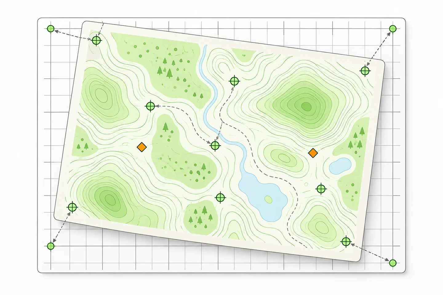
A scanned map is an image until its pixels are tied to coordinates. In QGIS, georeferencing makes the scan usable alongside other spatial layers. The main decisions are which locations to trust, how to spread control points across the sheet, and how to check the output away from those points. A close fit at the controls alone does not prove that the whole map is accurate.
Prepare the scan and its reference
Keep the original image and work on a copy. Inspect the sheet at a useful zoom: grid marks and their labels must be legible, and no cropped edge should remove coordinates you need. If a map was scanned in several pieces, handle each piece separately unless you can assemble them reliably first. The QGIS scanned-map lesson advises using as few scan sections as practical and keeping colour when it helps distinguish features.
Find a source of known positions before placing any points. A printed coordinate grid is useful because its crosses belong to the scanned map. An already georeferenced raster or vector layer can also provide positions where it shows the same identifiable features. Check its coverage, provenance and coordinate reference system (CRS). An attractive overlay is weak evidence if the reference layer is misplaced or the feature has changed since the map was drawn.
Read the map margin, legend and accompanying records for its projection and datum. Write down the CRS of the printed coordinates, the reference layer and the intended output. They need not be identical. The QGIS projection guide distinguishes a layer's assigned CRS from the project CRS used to display layers together. Setting a project CRS cannot repair coordinates interpreted under the wrong source CRS. If the map's CRS is uncertain, resolve that uncertainty before treating the result as spatial evidence.
Place ground control points
Open Layer → Georeferencer and load the working scan. With Add GCP Point, click a precise image location and supply its map coordinates. For a printed grid, zoom in, click the centre of a cross, enter its labelled values and specify the point's CRS. With a reference layer, click the matching feature in the scan and use From map canvas to select it on the existing map. The Georeferencer guide describes both methods.
Prefer unambiguous locations: clear grid intersections, identified building corners or stable bridge structures. A broad road centre, an approximate river bend or a junction altered since the scan was made is harder to match. Historical maps may also simplify or displace features. Exclude a point when you cannot identify the same place confidently in both sources; a precise click on the wrong feature still gives a wrong coordinate.
Spread points toward the corners and edges as well as through the interior. A cluster around one settlement may fit there while leaving the rest of the sheet poorly constrained. Use more than the transformation's minimum where reliable points are available, and reserve some suitable locations for checks after fitting. Before running the transformation, inspect the GCP table for swapped eastings and northings, a neighbouring grid cross, an incorrect CRS or a mismatched feature. Save the points with Save GCP Points As so the pairs can be reopened and corrected.
Choose a transformation that suits the sheet
Linear positions and uniformly scales a good-quality raster without changing its pixels; it writes a world file. Helmert adds rotation. Polynomial 1 can also account for differing scale and shear while preserving straight lines. Higher-order polynomials can model systematic curvature, while thin plate spline can accommodate local deformation. These flexible choices need more, well-distributed points and can distort regions between or beyond them. The QGIS transformation descriptions give the minimum GCP requirements and explain the trade-offs.
Start with the least flexible method that describes the scan's condition. A flat sheet does not need a complex warp to conceal one bad coordinate. Check suspect points and the source map first. A torn, stretched or photographed map may justify a more flexible fit, but only if independent checkpoints show that the result is useful where you need it. Record the reason for the choice, not just the displayed error figure.
In Transformation settings, select the target CRS and, for a method that creates a new raster, an output path and resampling method. Nearest neighbour retains original pixel values but may make linework appear jagged; interpolating methods can look smoother. The Linear world-file option leaves the image pixels unchanged. Enable Load in project when done if you want to inspect the result immediately. Keep the source scan regardless of the output method.
Check the fit beyond its controls
Residuals in the GCP table compare entered control positions with positions predicted by the fitted transformation. Look at both size and direction. One large residual may signal a typing error, an inaccurate click or a false match. A spatial pattern can point to weak coverage or distortion in the paper map. Investigate the cause before removing a point. Deleting a valid but awkward control solely to improve the summary figure can hide a real limitation.
The controls are not independent proof of accuracy. A flexible transformation can closely match them while bending the spaces between. Examine the locations held back as checkpoints: compare their positions on the output with printed grid coordinates or a trusted reference layer. Include an interior point and points near edges where the fit is weak. Note the direction and approximate size of each mismatch in units useful for your task. Decide what tolerance is acceptable from the map's scale, source quality and intended use rather than adopting a universal threshold.
For a visual check, place the output over a reference layer and adjust transparency, then zoom in at specific checkpoints. Broad alignment can hide local displacement. Conversely, a difference at one feature may reflect a rebuilt road, a changed shoreline or limited precision in the original drawing. Compare several stable locations before changing sound GCPs to force one feature into alignment. Keep those observations with the points file so another reader can see where the raster is dependable.
Work through a printed-grid example
The QGIS training lesson uses a scanned Finnish map with printed grid crosses in EPSG:2392, KKJ / Finland zone 2, while its project uses EPSG:3067, ETRS89 / TM35FIN(E,N). This is a useful reminder that the coordinates read from a sheet and the CRS used to display a project serve different purposes. For that map, a practical sequence is:
- Keep the supplied scan intact. Record the printed-grid CRS and the project CRS, then open a working copy in Georeferencer.
- Enter a clearly labelled grid cross and add readable crosses across the sheet. Check each value against the printed grid spacing.
- Leave several crosses out of the GCP set for later checks. Save the point file and note the transformation, target CRS, resampling method and output path.
- Inspect the residuals, run the transformation and compare the output at the unused crosses. Use the lesson's reference imagery as a further visual check where features can be matched confidently.
Save the result and its limitations
After Start georeferencing, confirm that the output opens in the intended CRS, covers the expected area and agrees at the reserved checkpoints. Retain the original scan, saved GCPs, output raster and a short record of the reference data, transformation and check results. QGIS can generate a PDF report with transformation details and residual information. State where alignment is adequate for your purpose and where paper distortion, uncertain source coordinates or changes on the ground limit interpretation.